Introduction to R

Overview

Teaching: 90 min
Exercises: 10 min

Questions

What are R and R Studio?

How do I write code in R?

How do I work with different types of data in R?

Objectives

To become oriented with R and R Studio.

To understand an R object and its class

To write logical comparisons between objects

To differentiate vectors, lists, and data frames

To subset R objects

Introduction to R and RStudio
Objects and Assignment
Data Types
Data Structures
Subsetting Data

Bonus: why learn to program?

Share why you’re interested in learning how to code.

Solution:

There are lots of different reasons, including to perform data analysis and generate figures. I’m sure you have morespecific reasons for why you’d like to learn!

Introduction to R and RStudio

Back to top

Over this workshop, we will be testing the hypothesis that a country’s life expectancy is related to the total value of its finished goods and services, also known as the Gross Domestic Product (GDP). To test this hypothesis, we’ll need two things: data and a platform to analyze the data.

You already downloaded the data. But what platform will we use to analyze the data? We have many options!

We could try to use a spreadsheet program like Microsoft Excel or Google sheets that have limited access, less flexibility, and don’t easily allow for things that are critical to “reproducible” research, like easily sharing the steps used to explore and make changes to the original data.

Instead, we’ll use a programming language to test our hypothesis. Today we will use R, but we could have also used Python for the same reasons we chose R (and we teach workshops for both languages). Both R and Python are freely available, the instructions you use to do the analysis are easily shared, and by using reproducible practices, it’s straightforward to add more data or to change settings like colors or the size of a plotting symbol.

But why R and not Python?

There’s no great reason. Although there are subtle differences between the languages, it’s ultimately a matter of personal preference. Both are powerful and popular languages that have very well developed and welcoming communities of scientists that use them. As you learn more about R, you may find things that are annoying in R that aren’t so annoying in Python; the same could be said of learning Python. If the community you work in uses R, then you’re in the right place.

To run R, all you really need is the R program, which is available for computers running the Windows, Mac OS X, or Linux operating systems. You downloaded R while getting set up for this workshop.

To make your life in R easier, there is a great (and free!) program called RStudio that you also downloaded and used during set up. As we work today, we’ll use features that are available in RStudio for writing and running code, managing projects, installing packages, getting help, and much more. It is important to remember that R and RStudio are different, but complementary programs. You need R to use RStudio.

Bonus Exercise: Can you think of a reason you might not want to use RStudio?

Solution:

On some high-performance computer systems (e.g. Amazon Web Services) you typically can’t get a display like RStudio to open. If you’re at the University of Michigan and have access to Great Lakes, then you might want to learn more about resources to run RStudio on Great Lakes.

To get started, we’ll spend a little time getting familiar with the RStudio environment and setting it up to suit your tastes. When you start RStudio, you’ll have three panels.

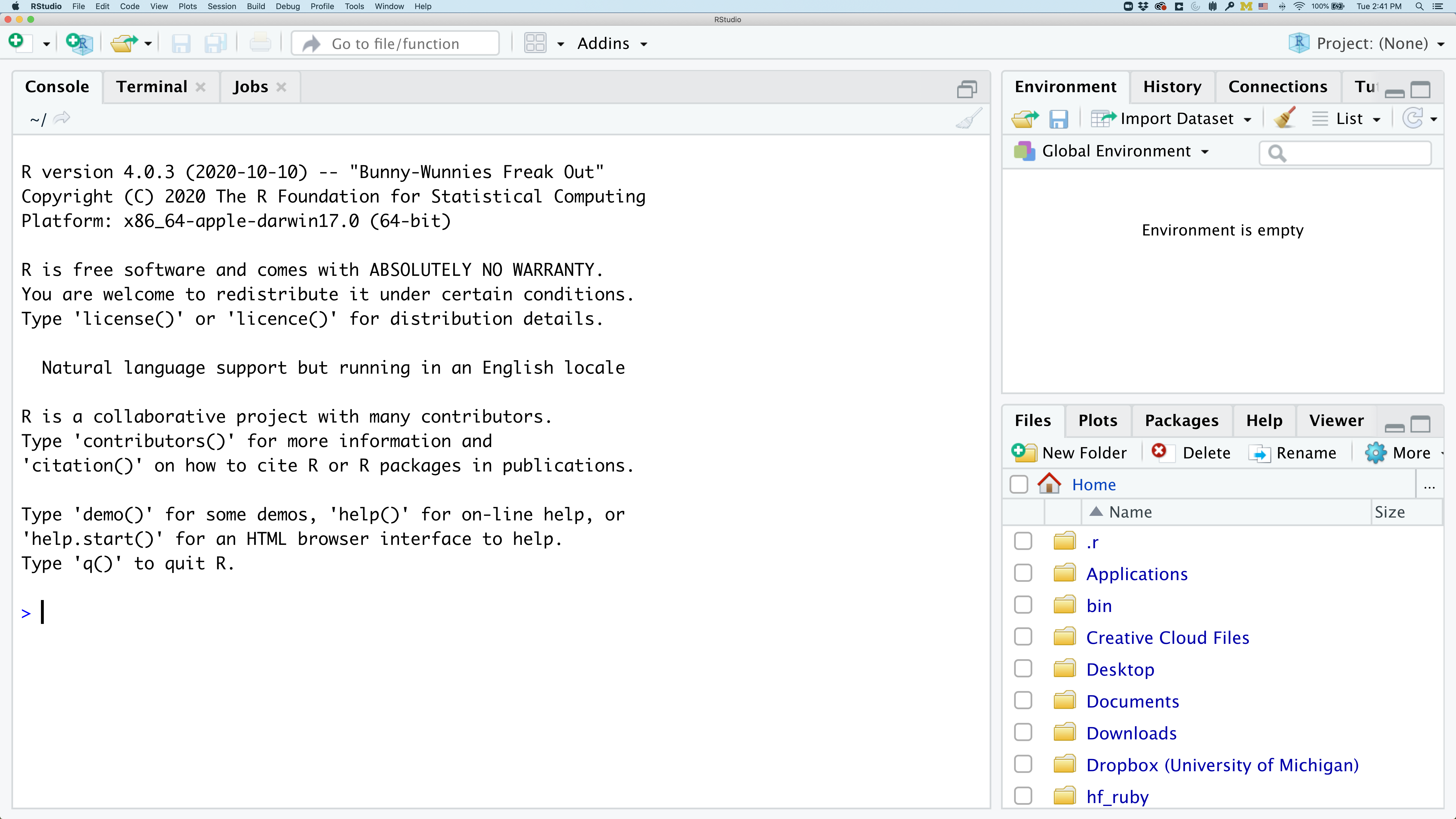
On the left you’ll have a panel with three tabs - Console, Terminal, and Jobs. The Console tab is what running R from the command line looks like. This is where you can enter R code. Try typing in 2+2 at the prompt (>). In the upper right panel are tabs indicating the Environment, History, and a few other things. If you click on the History tab, you’ll see the command you ran at the R prompt.

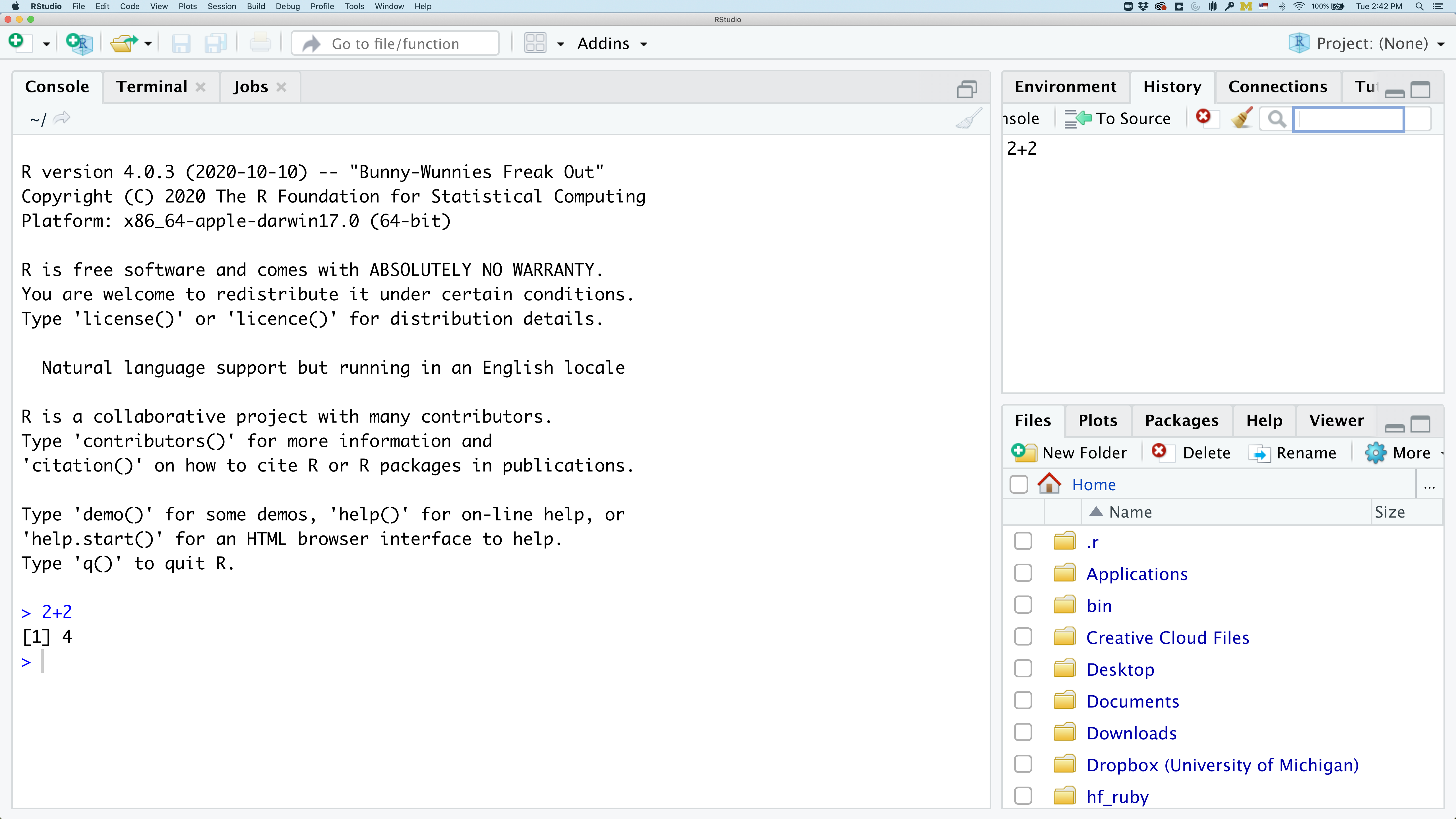
In the lower right panel are tabs for Files, Plots, Packages, Help, and Viewer. You used the Packages tab to install tidyverse.

We’ll spend more time in each of these tabs as we go through the workshop, so we won’t spend a lot of time discussing them now.

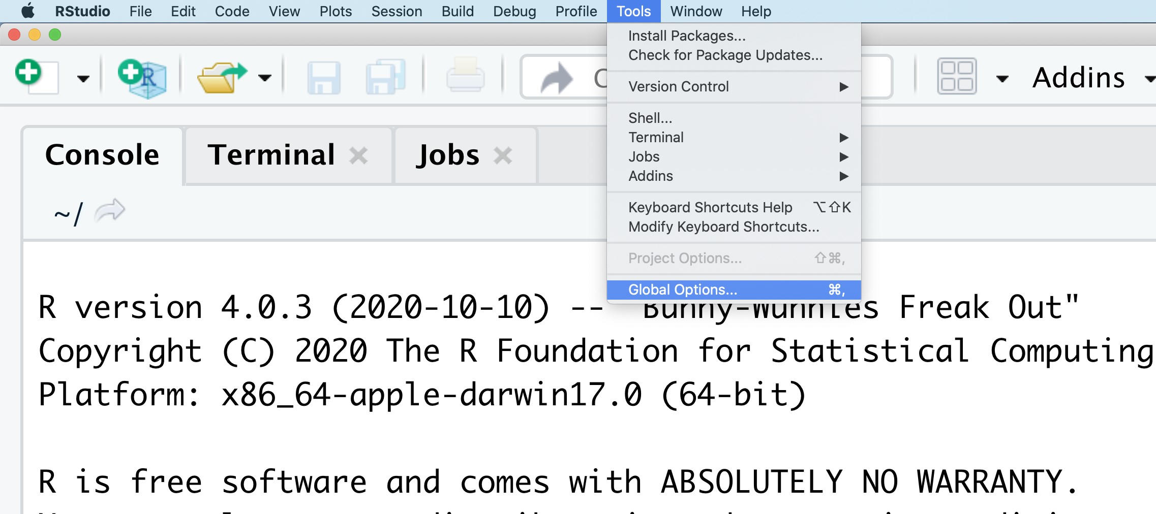
You might want to alter the appearance of your RStudio window. The default appearance has a white background with black text. If you go to the Tools menu at the top of your screen, you’ll see a “Global options” menu at the bottom of the drop down; select that.

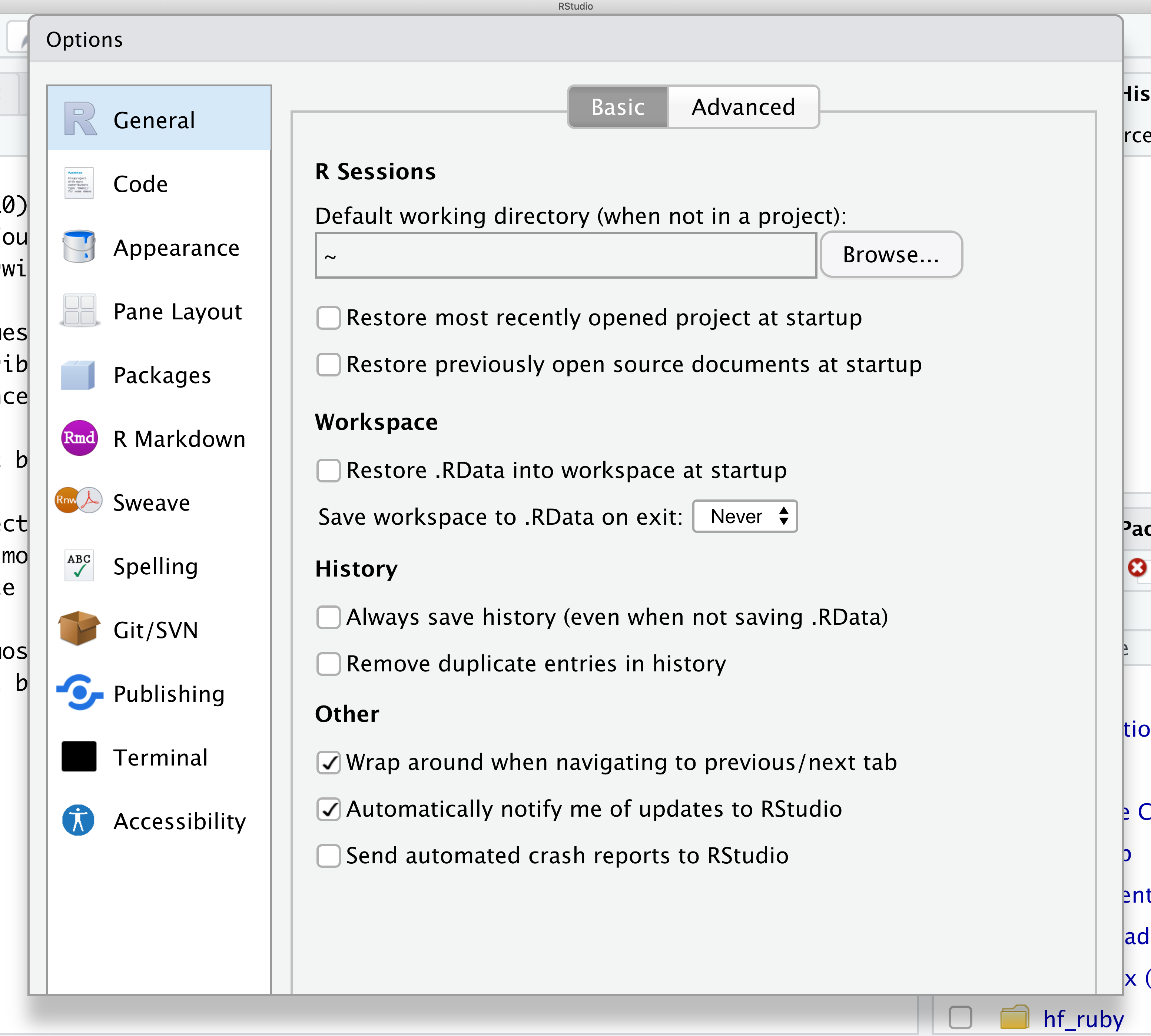
From there you will see the ability to alter numerous things about RStudio. Under the Appearances tab you can select the theme you like most. As you can see there’s a lot in Global options that you can set to improve your experience in RStudio. Most of these settings are a matter of personal preference.

However, you can update settings to help you to insure the reproducibility of your code. In the General tab, none of the selectors in the R Sessions, Workspace, and History should be selected. In addition, the toggle next to “Save workspace to .RData on exit” should be set to never. These setting will help ensure that things you worked on previously don’t carry over between sessions.

Let’s get going on our analysis!

One of the helpful features in RStudio is the ability to create a project. A project is a special directory that contains all of the code and data that you will need to run an analysis.

At the top of your screen you’ll see the “File” menu. Select that menu and then the menu for “New Project…”.

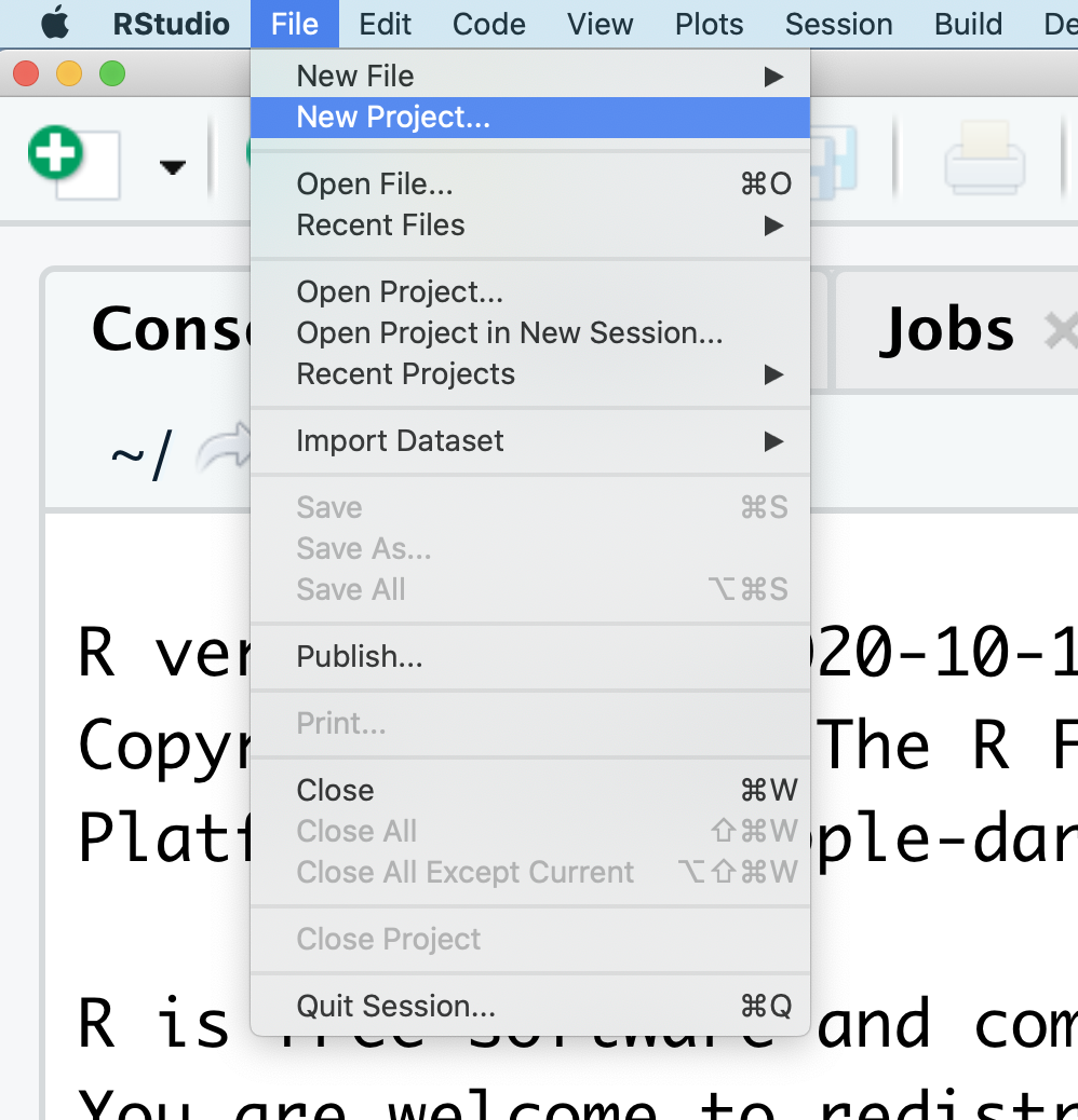
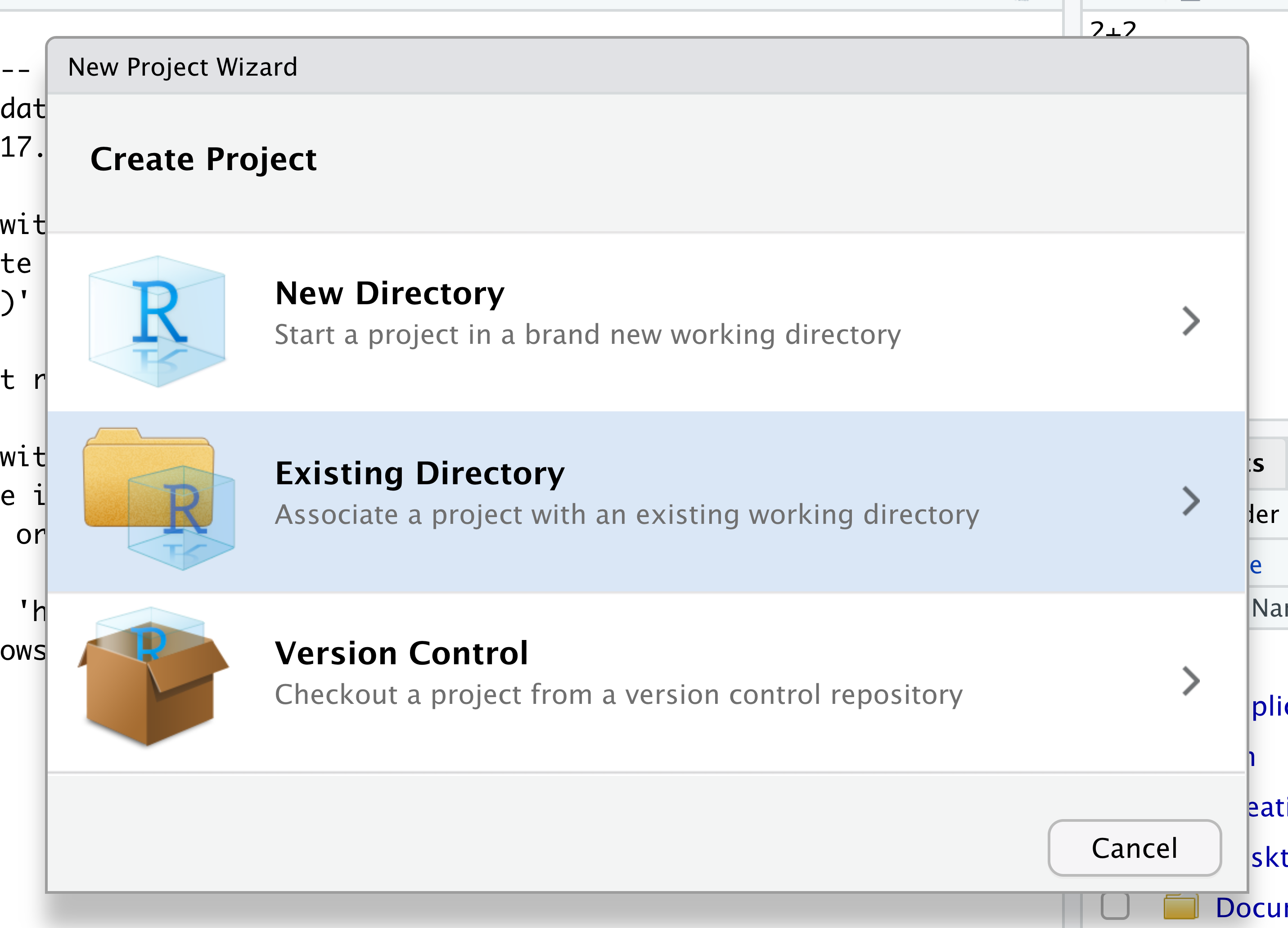
When the smaller window opens, select “Existing Directory” and then the “Browse” button in the next window.

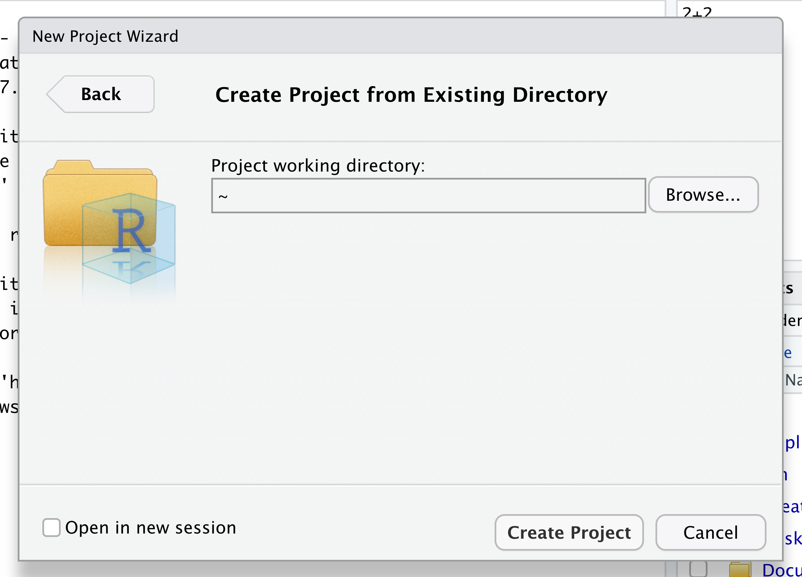
Navigate to the directory that contains your code and data from the setup instructions and click the “Open” button.

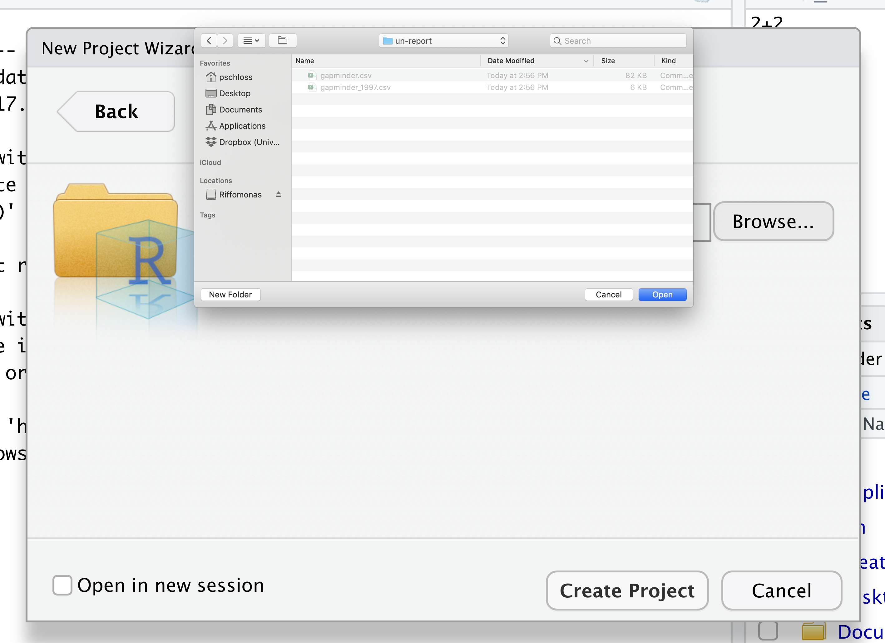
Then click the “Create Project” button.

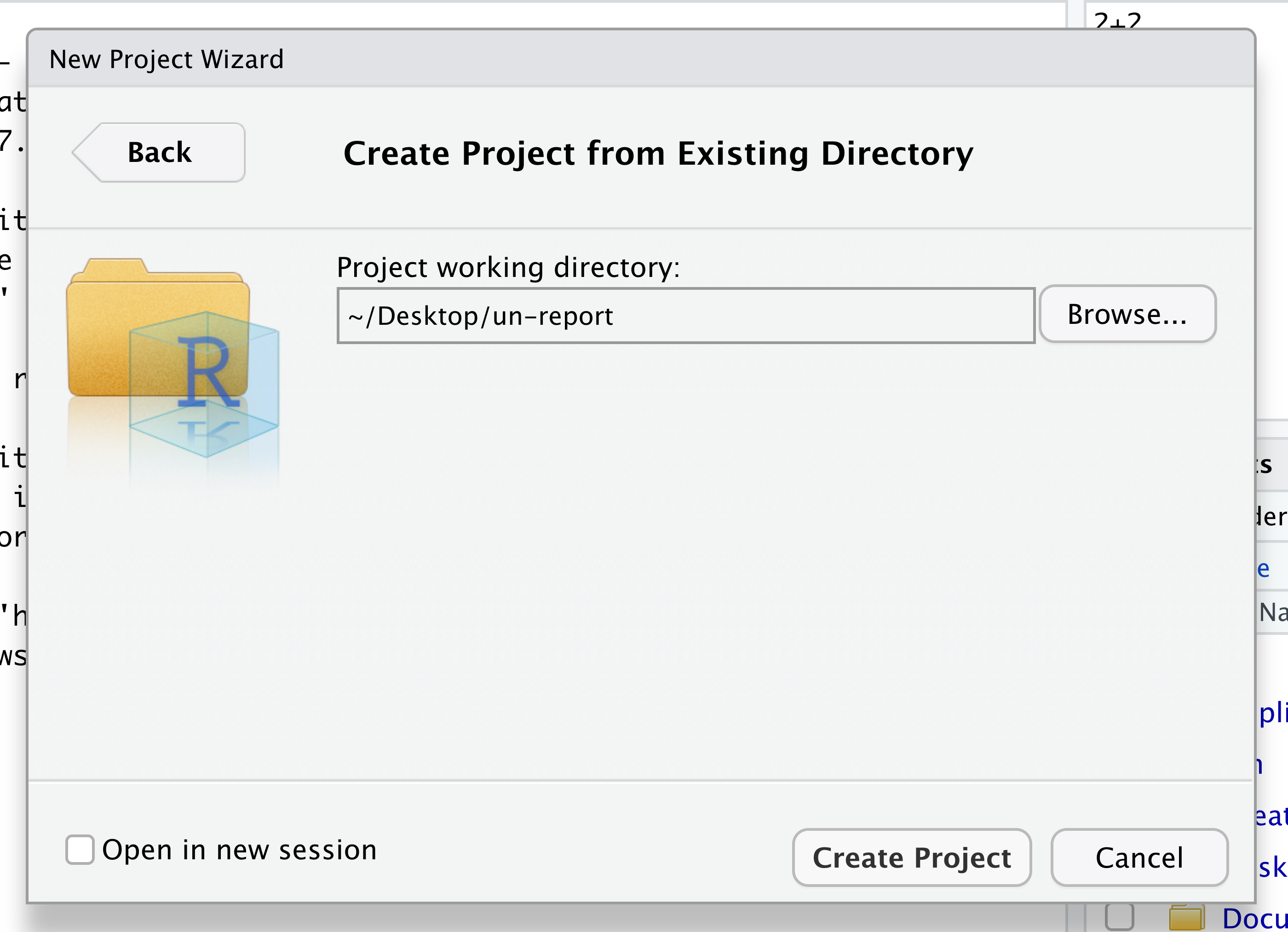
Did you notice anything change?

In the lower right corner of your RStudio session, you should notice that your Files tab is now your project directory. You’ll also see a file called un-report.Rproj in that directory.

From now on, you should start RStudio by double clicking on that file. This will make sure you are in the correct directory when you run your analysis.

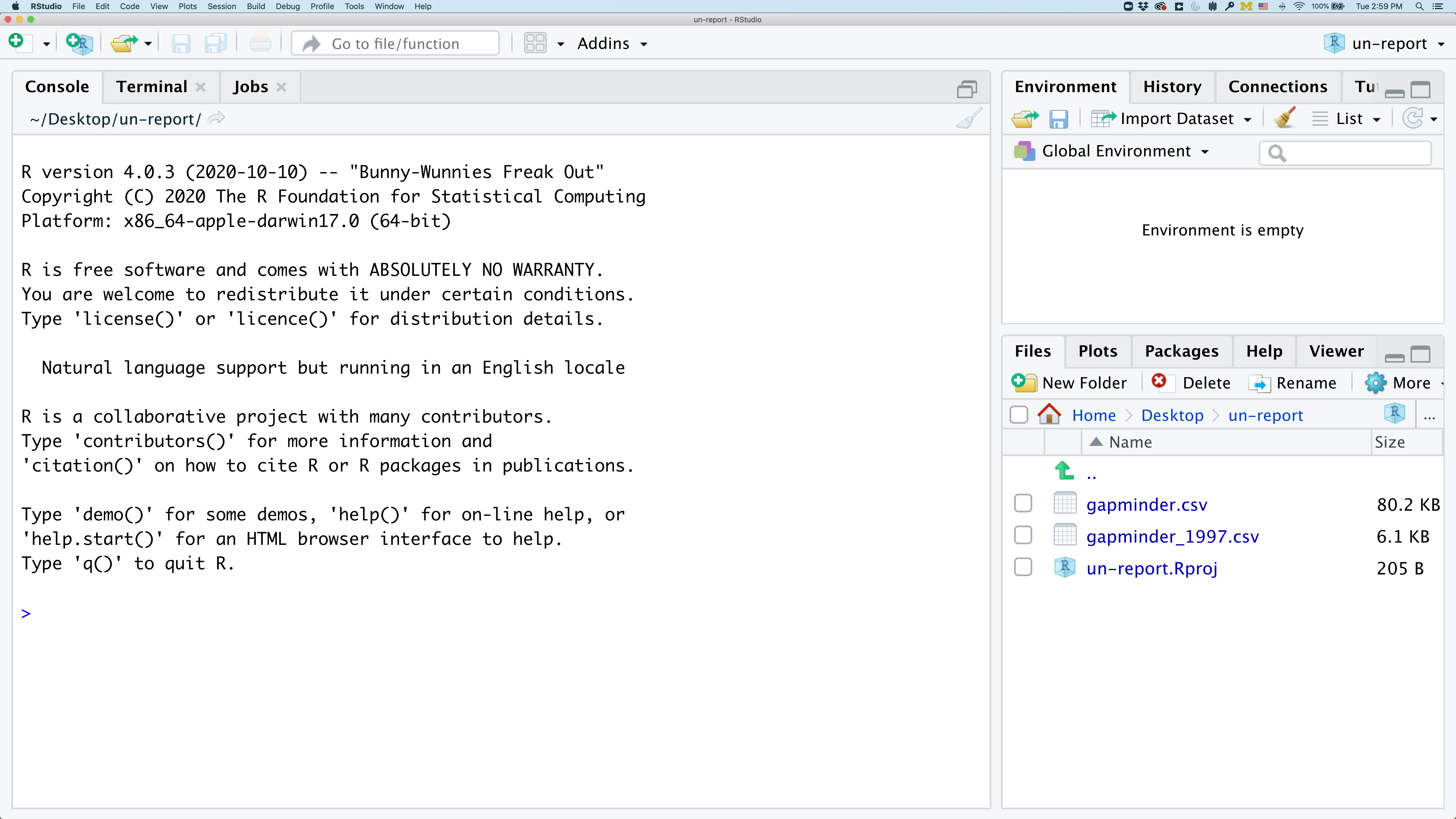
We’d like to create a file where we can keep track of our R code.

Back in the “File” menu, you’ll see the first option is “New File”. Selecting “New File” opens another menu to the right and the first option is “R Script”. Select “R Script”.

Now we have a fourth panel in the upper left corner of RStudio that includes an Editor tab with an untitled R Script. Let’s save this file as base_R.R in our project directory.

We will be entering R code into the Editor tab to run in our Console panel.

On line 1 of base_R.R, type 2+2.

With your cursor on the line with the 2+2, click the button that says Run. You should be able to see that 2+2 was run in the Console.

As you write more code, you can highlight multiple lines and then click Run to run all of the lines you have selected.

Objects and Assignment

Back to top

When we’re coding in R, we often want to assign a value, or a collection of values, to an object, which means we gave those values a name. To create an object in R, we’ll use the <- symbol, which is the assignment operator. It assigns values generated or typed on the right to objects on the left.

number_1 <- 2

number_2 <- 3

my_field <- "Microbiology"

Now we can see our obejcts in the Environment pane. An alternative symbol that you might see used as an assignment operator is the = but it is clearer to only use <- for assignment. We use this symbol so often that RStudio has a keyboard short cut for it: Alt+- on Windows, and Option+- on Mac. You can retrieve the values you stored by typing the name of the object.

number_1

[1] 2

number_1 + number_2

[1] 5

my_field

[1] "Microbiology"

Assigning values to objects

Try to assign values to some objects and observe each object after you have assigned a new value. What do you notice?
name <- "Ben"
name
age <- 26
age
name <- "Harry Potter"
name
Solution

When we assign a value to an object, the object stores that value so we can access it later. However, if we store a new value in an object we have already created (like when we stored “Harry Potter” in the name object), it replaces the old value. The age object does not change, because we never assign it a new value.

Guidelines on naming objects

You want your object names to be explicit and not too long.

They cannot start with a number (2x is not valid, but x2 is).

R is case sensitive, so for example, weight_kg is different from Weight_kg.

You cannot use spaces in the name.

There are some names that cannot be used because they are the names of fundamental functions in R (e.g., if, else, for; see here for a complete list). If in doubt, check the help to see if the name is already in use (?function_name).

It’s best to avoid dots (.) within names. Many function names in R itself have them and dots also have a special meaning (methods) in R and other programming languages.

It is recommended to use nouns for object names and verbs for function names.

Be consistent in the styling of your code, such as where you put spaces, how you name objects, etc. Using a consistent coding style makes your code clearer to read for your future self and your collaborators. One popular style guide can be found through the tidyverse.

Bonus Exercise: Bad names for objects

Try to assign values to some new objects. What do you notice? After running all four lines of code bellow, what value do you think the object Flower holds?
1number <- 3
Flower <- "marigold"
flower <- "rose"
favorite number <- 12
Solution

Notice that we get an error when we try to assign values to 1number and favorite number. This is because we cannot start an object name with a numeral and we cannot have spaces in object names. The object Flower still holds “marigold.” This is because R is case-sensitive, so running flower <- "rose" does NOT change the Flower object. This can get confusing, and is why we generally avoid having objects with the same name and different capitalization.

If we want to store a collection of values, we’ll need to use the c() (for “combine”) function, which combines values into something we call a vector. Let’s make a vector of numbers, and a vector of words (we call them “strings” in R)

my_num_vec <- c(1, 2, 3)

my_num_vec

[1] 1 2 3

my_name_vec <- c("Dog", "Cat", "Bird")

my_name_vec

[1] "Dog"  "Cat"  "Bird"

In R, functions will have a name (in this case, c), and then parentheses. Inside the parentheses are our arguments.

We can also add vectors together.

my_num_vec2 <- c(2,4,6)

my_num_vec + my_num_vec2

[1] 3 6 9

my_num_vec + my_name_vec

Error in my_num_vec + my_name_vec: non-numeric argument to binary operator

Oh no! We got an error from that last line of code. Don’t panic - errors are normal and are meant to help us. In order to understand this error, we need to discuss data types.

Data Types

Back to top

Every value in R has a type. We can ask what the datatype of an object is using another function, typeof().

typeof(my_num_vec)

[1] "double"

typeof(my_name_vec)

[1] "character"

Our vector of numbers is the type double, which you’ll also see written as numeric. The data type of our name vector is character. There are five main data types in R: double, integer, complex, logical, and character. Today, we’re only going to worry about double (numeric), character, and logical types. Logical types represent TRUE and FALSE.

my_logic_vec <- c(TRUE, FALSE, TRUE)

typeof(my_logic_vec)

[1] "logical"

Pro-tip

We don’t need to write out the full word TRUE or FALSE; we can also use T or F. R will not accept true or t. I like writing out the full word to make my code as clear as possible.

The data type of a vector determines what sort of functions we can use it in. For example, we can add two numerical vectors together, but we cannot add a character vector to a numeric vector. R is strict about these rules, and will give us errors if we try. Let’s see our last error again:

my_num_vec + my_name_vec

Error in my_num_vec + my_name_vec: non-numeric argument to binary operator

R is telling us it cannot add these vectors together, because we gave it a non-numeric (character) argument.

Data Structures

Back to top

The way we organize pieces of data in R is called a data structure. Luckily, we’ve already learned about one data structure - the vector! A vector is an organized list of values which have the same data type. What happens if we try to make a vector with a combination of data types?

mixed_vector <- c(2, TRUE, "Word")

mixed_vector

[1] "2"    "TRUE" "Word"

typeof(mixed_vector)

[1] "character"

All of the values in our mixed_vector have become characters. We can spot characters because they have “” around them. Converting between types is called coercion in R. Character is the most general data type, because while any number or logical value can be represented as a word, most words cannot be represented as numbers. We can coerce objects to different types, using functions that start with as. However, if R cannot figure out how to convert a value, it will return NA instead, and give you a warning.

as.character(my_num_vec)

[1] "1" "2" "3"

as.numeric(my_logic_vec)

[1] 1 0 1

as.numeric(my_name_vec)

Warning: NAs introduced by coercion

[1] NA NA NA

What if we want an object in R that can hold multiple different types of data? For this, we have a specialized data structure in R, called a list. While we make vectors using the c() function, we make lists using the list() function.

my_list <- list(2, c(TRUE,FALSE), "Word")

my_list

[[1]]
[1] 2

[[2]]
[1]  TRUE FALSE

[[3]]
[1] "Word"

If we click on my_list in the environment pane, we can see what values it stores. Notice that none of the values underwent coercion, unlike in our vector. Lists can hold anything, including vectors and even other lists.

While vectors and lists are important data structures, as microbiologists, most of the time we work with tabular data. In R, tabular data is represented by a structure called a data.frame. Like lists, data.frames can hold multiple data types. We can make a data.frame from scratch using the data.frame() function.

micro_df <- data.frame(species = c("Ecoli", "Bsubtilis", "Saureus"),
                       gram_pos = c(FALSE, TRUE, TRUE),
                       genome_mbp = c(5, 4.2, 2.8))

micro_df

    species gram_pos genome_mbp
   Ecoli    FALSE        5.0
Bsubtilis     TRUE        4.2
 Saureus     TRUE        2.8

Data.frames are organized by columns (variables) and rows (observations). To view data.frames, we can print them in the console by typing their name, or clicking on them in the Environment pane. Data.frames come with some rules:

Every column needs to have the same number of rows
Each column is a single data type
Column names should be valid object names in R, so avoid spaces, special characters, and starting with numbers (there are workarounds but we should avoid them).

Subsetting Data

Back to top

Often, we want to access specific values from data structure in R. There are six different ways we can subset any kind of object, and three different subsetting operators for the different data structures.

Let’s start with vectors.

x <- c(5.4, 6.2, 7.1, 4.8, 7.5)
x

[1] 5.4 6.2 7.1 4.8 7.5

Atomic vectors

In R, simple vectors containing character strings, numbers, or logical values are called atomic vectors because they can’t be further simplified.

Accessing elements using their indices

Back to top

To extract elements of a vector we can use square brackets [] and give their corresponding index, starting from one:

x[1]

[1] 5.4

x[4]

[1] 4.8

It may look different, but the square brackets operator is a function. For vectors (and matrices), it means “get me the nth element”.

We can ask for multiple elements at once, by putting a vector in the brackets:

x[c(1, 3)]

[1] 5.4 7.1

Or slices of the vector:

x[1:4]

[1] 5.4 6.2 7.1 4.8

the : operator creates a sequence of numbers from the left element to the right.

1:4

[1] 1 2 3 4

c(1, 2, 3, 4)

[1] 1 2 3 4

We can ask for the same element multiple times:

x[c(1,1,3)]

[1] 5.4 5.4 7.1

If we ask for an index beyond the length of the vector, R will return a missing value:

x[6]

[1] NA

This is a vector of length one containing an NA, whose name is also NA.

If we ask for the 0th element, we get an empty vector:

x[0]

numeric(0)

Vector numbering in R starts at 1

In many programming languages (C and Python, for example), the first element of a vector has an index of 0. In R, the first element is 1.

Skipping and removing elements

Back to top

If we use a negative number as the index of a vector, R will return every element except for the one specified:

x[-2]

[1] 5.4 7.1 4.8 7.5

We can skip multiple elements:

x[c(-1, -5)]  # or x[-c(1,5)]

[1] 6.2 7.1 4.8

To remove elements from a vector, we need to assign the result back into the variable:

x <- x[-4]
x

[1] 5.4 6.2 7.1 7.5

Bonus Exercise: Subsetting by Number

Given the following code:
x <- c(5.4, 6.2, 7.1, 4.8, 7.5)
print(x)
[1] 5.4 6.2 7.1 4.8 7.5
Come up with at least 2 different commands that will produce the following output:
[1] 6.2 7.1 4.8
Solution
x[2:4]
[1] 6.2 7.1 4.8
x[-c(1,5)]
[1] 6.2 7.1 4.8
x[c(2,3,4)]
[1] 6.2 7.1 4.8

Subsetting by name

Back to top

We can extract elements by using their name, instead of extracting by index. To do so, we first need to give our vector names

x <- c(5.4, 6.2, 7.1, 4.8, 7.5)

names(x) <- c('a', 'b', 'c', 'd', 'e')

x[c("a", "c")]

  a   c 
5.4 7.1 

This is usually a much more reliable way to subset objects: the position of various elements can often change when chaining together subsetting operations, but the names will always remain the same!

Subsetting through logical operations

Back to top

We can also use any logical vector to subset:

x[c(FALSE, FALSE, TRUE, FALSE, TRUE)]

  c   e 
7.1 7.5 

Usually, we don’t want to type out all the TRUEs and FALSEs. Instead, we want to find data that match a specific condition. To do so, we use logical operators. We use these functions to compare values in R, and they return a logical value. Some common logical operators include == (“is equal to”), != (“is not equal to”), >/< (“is greater than/is lesser than”), and >=/<= (“is greater or equal to/is lesser or equal to”).

"A" == "B"

[1] FALSE

"b" != "A"

[1] TRUE

3 > 2

[1] TRUE

3 <= 2

[1] FALSE

We can use a logical operator on a vector, which produces a logical vector.

  a   b   c   d   e 
5.4 6.2 7.1 4.8 7.5 

x > 5

    a     b     c     d     e 
 TRUE  TRUE  TRUE FALSE  TRUE 

As such, we can use the results of a logical comparison to subset a vector.

x[x > 7]

  c   e 
7.1 7.5 

Breaking it down, this statement first evaluates x>7, generating a logical vector c(FALSE, FALSE, TRUE, FALSE, TRUE), and then selects the elements of x corresponding to the TRUE values.

We can use == to mimic the previous method of indexing by name (remember you have to use == rather than = for comparisons):

x[names(x) == "a"]

  a 
5.4 

Tip: Combining logical conditions

We often want to combine multiple logical criteria. We can link logical operators using the & and | operators:

&, the “logical AND” operator: returns TRUE if both the left and right are TRUE.

|, the “logical OR” operator: returns TRUE, if either the left or right (or both) are TRUE.

You may sometimes see && and || instead of & and |. These two-character operators only look at the first element of each vector and ignore the remaining elements. In general you should not use the two-character operators in data analysis; save them for programming, i.e. deciding whether to execute a statement.

!, the “logical NOT” operator: converts TRUE to FALSE and FALSE to TRUE. It can negate a single logical condition (eg !TRUE becomes FALSE), or a whole vector of conditions(eg !c(TRUE, FALSE) becomes c(FALSE, TRUE)).

Additionally, you can compare the elements within a single vector using the all function (which returns TRUE if every element of the vector is TRUE) and the any function (which returns TRUE if one or more elements of the vector are TRUE).

Bonus Exercises

Given the following code:
x <- c(5.4, 6.2, 7.1, 4.8, 7.5)
names(x) <- c('a', 'b', 'c', 'd', 'e')
print(x)
  a   b   c   d   e 
5.4 6.2 7.1 4.8 7.5 
Write a subsetting command to return the values in x that are greater than 4 and less than 7.
Solution to challenge 2
x_subset <- x[x<7 & x>4]
print(x_subset)
  a   b   d 
5.4 6.2 4.8 

Subsetting Lists

Back to top

Now we’ll introduce some new subsetting operators. There are three functions used to subset lists. We’ve already seen one of these when learning about atomic vectors ([), and we’ll learn two more, ([[), and ($).

Using [ will always return a list. We can check the data structure of an object using the class() function. If you want to subset a list, but not extract an element, then you will likely use [.

my_list

[[1]]
[1] 2

[[2]]
[1]  TRUE FALSE

[[3]]
[1] "Word"

class(my_list)

[1] "list"

my_list[1]

[[1]]
[1] 2

class(my_list[1])

[1] "list"

This returns a list with one element.

To extract individual elements of a list, you need to use the double-square bracket function: [[.

my_list[[2]]

[1]  TRUE FALSE

class(my_list[[2]])

[1] "logical"

Notice that now the result is a vector, not a list.

You can’t extract more than one element at once:

my_list[[1:2]]

Error in my_list[[1:2]]: subscript out of bounds

Nor use it to skip elements:

my_list[[-1]]

Error in my_list[[-1]]: invalid negative subscript in get1index <real>

We can also extract using names. We’ll first need to add names to our list.

names(my_list)

NULL

names(my_list) <- c("a","b","c")

my_list

$a
[1] 2

$b
[1]  TRUE FALSE

$c
[1] "Word"

Now, let’s extract using the name of the first object:

my_list[["a"]]

[1] 2

The $ function is a shorthand way for extracting elements by name:

my_list$b

[1]  TRUE FALSE

Subsetting Data Frames

Back to top

Similar rules apply for data frames as with lists. However they are also two dimensional objects, so there are some differences.

[ with one argument will act the same way as for lists, where each list element corresponds to a column. The resulting object will be a data frame:

micro_df

    species gram_pos genome_mbp
   Ecoli    FALSE        5.0
Bsubtilis     TRUE        4.2
 Saureus     TRUE        2.8

micro_df[1]

    species
   Ecoli
Bsubtilis
 Saureus

Similarly, [[ will act to extract a single column as a vector:

micro_df[[1]]

[1] "Ecoli"     "Bsubtilis" "Saureus"

And $ provides a convenient shorthand to extract columns by name:

micro_df$species

[1] "Ecoli"     "Bsubtilis" "Saureus"

We can also index by both rows and columns. We’ll use the [ function, but instead provide 2 arguments, separated by a comma. The first will specify rows, and the second will specify columns. For example:

# Pull out the first row
micro_df[1,]

  species gram_pos genome_mbp
1   Ecoli    FALSE          5

# Pull out the second column
micro_df[,2]

[1] FALSE  TRUE  TRUE

# Pull out object at row 1, column two
micro_df[1,2]

[1] FALSE

If we subset a single row, the result will be a data frame (because the elements are mixed types).

But for a single column the result will be a vector.

Finally, we often want to select rows of a data frame that match a certain condition. To do this, we’ll combine skills we learned in subsetting and logical comparisons.

First, let’s select a specific column:

micro_df$genome_mbp

[1] 5.0 4.2 2.8

Then, let’s use it in a logical comparison:

micro_df$genome_mbp > 4

[1]  TRUE  TRUE FALSE

Finally, let’s use that logical vector to select rows from our data frame with the [ operator:

micro_df[micro_df$genome_mbp > 4]

    species gram_pos
   Ecoli    FALSE
Bsubtilis     TRUE
 Saureus     TRUE

Hmm. Did that do what we wanted? Our logical vector was TRUE TRUE FALSE. It looks like we selected the first two columns of the data frame, not the first two rows. Remember that the [ assume you’re selecting columns by default. If we want them to select rows, we need to add a ,

micro_df[micro_df$genome_mbp > 4,]

    species gram_pos genome_mbp
1     Ecoli    FALSE        5.0
2 Bsubtilis     TRUE        4.2

Perfect!

Challenge

Fix each of the following common data frame subsetting errors:

Extract observations collected for E. coli
  micro_df[micro_df$species = "Ecoli",]
Drop columns 2 and 3
  micro_df[,-2:3]
Extract the rows where the genome size is larger than 4.5 Mbp
  micro_df[micro_df$genome_mbp > 4.5]
Extract the first row, and the 2nd and 3rd columns
  micro_df[1, 2, 3]
Advanced: extract rows that contain information for B. subtilis or S. aureus
  micro_df[micro_df$species == "Bsubtilis" | "Saureus",]
Solution

Fix each of the following common data frame subsetting errors:

Extract observations collected for E. coli
  # micro_df[micro_df$species = "Ecoli",]
  micro_df[micro_df$species == "Ecoli",]
Drop columns 2 and 3
  # micro_df[,-2:3]
  micro_df[-c(2:3)]
Extract the rows where the genome size is larger than 4.5 Mbp
  # micro_df[micro_df$genome_mbp > 4.5]
  micro_df[micro_df$genome_mbp > 4.5,]
Extract the first row, and the 2nd and 3rd columns
  # micro_df[1, 2, 3]
  micro_df[1, c(2, 3)]
Advanced: extract rows that contain information for B. subtilis or S. aureus
  # micro_df[micro_df$species == "Bsubtilis" | "Saureus",]
  micro_df[micro_df$species == "Bsubtilis" | micro_df$species == "Saureus",]
  
  # Or if you're lazy...
  micro_df[micro_df$gram_pos,]

Bonus: If else statements

Often when we’re coding we want to control the flow of our actions. This can be done by setting actions to occur only if a condition or a set of conditions are met. Alternatively, we can also set an action to occur a particular number of times.

There are several ways you can control flow in R. For conditional statements, the most commonly used approaches are the constructs:

# if
if (condition is true) {
  perform action
}

# if ... else
if (condition is true) {
  perform action
} else {  # that is, if the condition is false,
  perform alternative action
}

Say, for example, that we want R to print a message if a variable x has a particular value:

x <- 8

if (x >= 10) {
  print("x is greater than or equal to 10")
}

x

[1] 8

The print statement does not appear in the console because x is not greater than 10. To print a different message for numbers less than 10, we can add an else statement.

x <- 8

if (x >= 10) {
  print("x is greater than or equal to 10")
} else {
  print("x is less than 10")
}

[1] "x is less than 10"

You can also test multiple conditions by using else if.

x <- 8

if (x >= 10) {
  print("x is greater than or equal to 10")
} else if (x > 5) {
  print("x is greater than 5, but less than 10")
} else {
  print("x is less than 5")
}

[1] "x is greater than 5, but less than 10"

Important: when R evaluates the condition inside if() statements, it is looking for a logical element, i.e., TRUE or FALSE. This can cause some headaches for beginners. For example:

x  <-  4 == 3
if (x) {
  "4 equals 3"
} else {
  "4 does not equal 3"
}

[1] "4 does not equal 3"

As we can see, the not equal message was printed because the vector x is FALSE

x <- 4 == 3
x

[1] FALSE

Challenge

Use an if() statement to print a suitable message reporting whether there are any records from B. subtilis in our micro_df. Some functions that we have learned but could be helpful > include any(), or nrow. Preview their help pages for hints using the ? function.
Solution

We will first see a solution which uses the nrow function. We first obtain a logical vector describing which element of micro_df$species is equal to Bsubtilis:
micro_df[(micro_df$species == "Bsubtilis"),]
Then, we count the number of rows of the data.frame micro_df that correspond to the “Bsubtilis”:
bac_row_number <- nrow(micro_df[(micro_df$species == "Bsubtilis"),])
The presence of any record for the year “Bsubtilis” is equivalent to the request that rows"Bsubtilis"_number is one or more:
bac_row_number >= 1
Putting all together, we obtain:
if(nrow(micro_df[(micro_df$species == "Bsubtilis"),]) >= 1){
   print("Record(s) for Bsubtilis found.")
}
All this can be done more quickly with any(). The logical condition can be expressed as:
if(any(micro_df$species == "Bsubtilis")){
   print("Record(s) for Bsubtilis found.")
}

Did anyone get a warning message like this?

Error in if (micro_df$species == "Bsubtilis") {: the condition has length > 1

The if() function only accepts singular (of length 1) inputs, and therefore returns an error when you use it with a vector. The if() function will still run, but will only evaluate the condition in the first element of the vector. Therefore, to use the if() function, you need to make sure your input is singular (of length 1).

Tip: Built in ifelse() function

R accepts both if() and else if() statements structured as outlined above, but also statements using R’s built-in ifelse() function. This function accepts both singular and vector inputs and is structured as follows:
# ifelse function
ifelse(condition is true, perform action, perform alternative action)
where the first argument is the condition or a set of conditions to be met, the second argument is the statement that is evaluated when the condition is TRUE, and the third statement is the statement that is evaluated when the condition is FALSE.
y <- -3
ifelse(y < 0, "y is a negative number", "y is either positive or zero")
[1] "y is a negative number"

Tip: any() and all()

The any() function will return TRUE if at least one TRUE value is found within a vector, otherwise it will return FALSE. This can be used in a similar way to the %in% operator. The function all(), as the name suggests, will only return TRUE if all values in the vector are TRUE.

Key Points

R is a free programming language used by many for reproducible data analysis.

The class of an object describes what type of data is holds

We can use numbers, names, or logical values to subset data

previous episode

Cornell Carpentries Curriculum

next episode

Introduction to R

Overview

Contents

Bonus: why learn to program?

Solution:

Introduction to R and RStudio

But why R and not Python?

Solution:

Objects and Assignment

Assigning values to objects

Solution

Guidelines on naming objects

Bonus Exercise: Bad names for objects

Solution

Data Types

Pro-tip

Data Structures

Subsetting Data

Atomic vectors

Accessing elements using their indices

Vector numbering in R starts at 1

Skipping and removing elements

Bonus Exercise: Subsetting by Number

Solution

Subsetting by name

Subsetting through logical operations

Tip: Combining logical conditions

Bonus Exercises

Solution to challenge 2

Subsetting Lists

Subsetting Data Frames

Challenge

Solution

Bonus: If else statements

Challenge

Solution

Tip: Built in ifelse() function

Tip: any() and all()

Key Points

previous episode

next episode

Tip: Built in `ifelse()` function

Tip: `any()` and `all()`